Memento mori
and remember that all monitoring programs end at some point
---
I don't remember exactly when I had the idea I describe in the following, but I clearly remember I had a conversation about it with Ryan Chisholm (now at the National University of Singapore) while attending the SIAM meeting in San Diego in the summer of 2013. Marc Mangel was invited, but he could not go. The organizer of the special session on spatial ecology asked Marc if he had a postdoc to recommend as a substitute for him and he recommended me. Semi-surreal experience with only the five people scheduled to give talks present in the room and a couple of them were busy checking emails. I had a very good time, though.
As a side note, I recently had a look at the slides of the talk I gave at SIAM 2013, and there are at least a couple of ideas that could become papers, one on density dependent growth at different spatial scales (which I had partially developed Vincenzi, S. et al. 2010 Detection of density-dependent growth at two spatial scales in marble trout (Salmo marmoratus) populations. Ecol. Freshw. Fish 19, 338–347) and one on rapid genetic differentiation in fish populations living in fragmented habitats. Ryan also talked about his recent (at the time) trip to Cuba and he convinced me - it was not too hard - to visit the island. I went to Cuba for the first time in November 2013, I fell in love with La Habana, and I have been there other 2 times, the last one (October-November 2016) also presenting my research at the Centro de Investigaciones Marinas of Universidad de La Habana.

In La Habana at the beginning of November 2016, humidity at 150% and not too happy about it.
The main idea is this: most monitoring programs start with no end in sight (funding is largely determining the duration of the program) and often with different goals that require vastly different amount of data, for instance estimating average survival or growth rates may require 3 to 5 years of data for salmonids (my model system), while estimating the effects on population dynamics or life-history traits of extreme events such as floods, fires, drought, hurricanes, tautologically require at least the occurrence of one extreme event across multiple populations or multiple rare events in one population (otherwise it is not possible to test hypotheses sensu Platt, J. R. 1964 Strong inferences. Science 146, 347–353.)
How can we define an event as extreme? As I wrote in a 2014 paper (Vincenzi, S. 2014 Extinction risk and eco-evolutionary dynamics in a variable environment with increasing frequency of extreme events. J. R. Soc. Interface 11, 20140441), "[...] extreme events may be defined in terms of extreme values of a continuous variable on the basis of the available climate record (e.g. temperature, precipitation levels) or in the form of a discrete (point) perturbation, such as a hurricane or a heavy storm. This latter category also includes environmental extremes such as unusually big fires, aseasonal floods or rain-on-snow events.". Extremeness includes and goes beyond rarity, and we can assume extreme events to be defined as extreme have recurrence intervals that are longer than the generation time of the species we are investigating.
It follows that if we are interested in the effects of rare events, the minimum duration of the monitoring program is dictated by the expected recurrence interval of the extreme event, but if in absence of extreme events (that is, extreme events are not expected for that species/population) we want to estimate "reliable" average survival and growth rates (which along with recruitment represent the main axes of variation in species' vitals rates and are essential for the development of any self-respecting model of population dynamics) is unclear for how long we need to go on with the monitoring program. I am not the first one to think about this problem in conservation biology, see for instance Chapter 23 of "Design and Analysis of Long-term Ecological Monitoring Studies" (many editors): "Choosing among long-term ecological monitoring programs and knowing when to stop" by Hugh P. Possingham, Richard A. Fuller, and Liana N. Joseph, or Gerber, L. R., M. Beger, M. A. McCarthy, et al. 2005. A theory for optimal monitoring of marine reserves. Ecol Lett 8, 829–837.
In practical terms, I was interested in estimating how stable were the estimates of average, maximum, and minimum (for a sampling interval) survival rates, and somatic growth rates (i.e., body growth) over time in populations of marble, brown, and rainbow trout living in Western Slovenian streams. Briefly, two populations of marble, one of brown, and one of rainbow trout were sampled bi-annually (June and September) between 2004 and 2014 (monitoring is still ongoing, but for various reasons in this study I only included data up to 2014). Those populations were not affected by extreme events since the start of the monitoring program. It is tricky to assess what's "stable" since we estimate rates or probabilities, thus we inevitably have uncertainty in the estimation, but let's put aside this thorny problem for a moment with the assumption we can at least qualitatively see or define "by look" what's stable or not.
Without getting deep into the gory details (and there are many), what I did was to fit capture-recapture models (fish were tagged when bigger than 115 mm) of survival and growth (using von Bertalanffy's growth models) with data available after 3, 4, 5 (and so on) years since the start of the monitoring program. For growth, I used two von Bertalanffy's models, one with random effects (see Vincenzi, S. et al. 2014 Determining individual variation in growth and its implication for life-history and population processes using the Empirical Bayes method. PLoS Comput. Biol. 10, e1003828) and one "classic", that is without individual random effects (I simply used the nls function in R, thus each data point is - wrongly - assumed to be coming from different individuals). For survival, I fitted models Phi(~1) (constant survival) and Phi(~time) (survival varying for each sampling occasion) with different models of probability of capture. With Phi(~time) models, I had the goal to estimate the maximum and minimum survival probabilities over sampling intervals (apart from statistical noise or use of different models of probability of capture, over time maximum survival probability for a sampling interval cannot become smaller and minimum survival probability cannot become bigger).
These are the results for growth, I took asymptotic length (of the average fish) as estimated response variable (estimates with classic nonlinear regression (dot symbol) and estimates with the model with random effects (triangle)), x-axis is the last year of sampling (for, say, 2006, I only keep the data for up to 2006, for 2010 up to 2010, and every time I re-fit models with the corresponding datasets). With the model with random effects, it takes 2 to 4 years to obtain a stable estimate. With the classic method, we need more years, and in some cases, the model gives wrong estimates, since outliers strongly pull the average growth trajectories in their direction (as I also discuss in the PLoSCompBio paper cited above and in another one currently under review). Vertical lines are standard errors of the estimate.
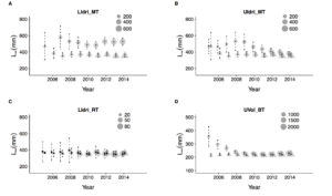
Estimates of asymptotic length using the classic method (dots) and the random-effects model (triangles). The size of symbols is proportional to sample size. LIdri_MT = marble trout in Lower Idrijca, UIdri_MT = marble trout in Upper Idrijca, LIdri_RT = rainbow trout in Lower Idrijca, UVol_BT = brown trout in Upper Volaja.
As I wrote in another paper currently under review: "The vBGF parameters can seldom be interpreted separately, especially when only a few older fish are measured; it follows that the analysis of the whole growth trajectories is necessary for understanding growth variation among individuals and cohorts". The second plot for growth shows the average growth trajectories using the random-effect models using data up to 2006 or up to 2014. Within populations and for all intents and purposes, the average growth trajectories are basically the same.
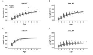
Average growth trajectories for the 4 salmonid populations estimated with data up to 2006 or up to 2014 with the random-effects model. LIdri_MT = marble trout in Lower Idrijca, UIdri_MT = marble trout in Upper Idrijca, LIdri_RT = rainbow trout in Lower Idrijca, UVol_BT = brown trout in Upper Volaja.
The last plot is about survival. x-axis is again the last year of simulated sampling, dot is the estimate of average survival, up triangle is the maximum estimated survival for a sampling interval, down triangle is the minimum estimated survival for a sampling interval. The estimate of average survival is very stable after just 2 or 3 years (4 to 6 sampling occasions), except for rainbow trout since the small sample size makes the estimate vary quite a bit, as expected.
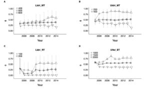
Dots are average survival probabilities (Phi(~1)), up and down triangles are maximum and minimum survival for sampling occasion (max and min estimates of Phi(~time)). LIdri_MT = marble trout in Lower Idrijca, UIdri_MT = marble trout in Upper Idrijca, LIdri_RT = rainbow trout in Lower Idrijca, UVol_BT = brown trout in Upper Volaja.
The main point and message to take home from this work are that in salmonid populations 2 or 3 years of data may be enough to get "stable" estimates of survival and average growth trajectories, the latter only if using a random-effects model of growth, but > 5 years are needed to estimate maximum and minimum survival probabilities in absence of extreme events (and potentially longer for minimum survival probabilities, as it can be seen in the panels for LIdri_MT and UIdri_MT).
Interesting, surprising, useful, worthy of publication in a conservation journal such as Biological Conservation, Animal Conservation, Conservation Biology?